Evaluation

Evaluation is important and a key process in a project completion. This evaluation is to present the  results of our system, for locating the trackable object position and track its (movement) repositioning over  time using mobile smartphones as  data collectors.  The  usability of the system relies  on  the results collected from  mobile smartphone over  time, more collection from  more users means better results and improving of accuracy. Accuracy in this context means predicting the position of the mobile smartphone in testbed 4.1 (PitLAB) as good  as possible at each direction as demonstrate in this  picture 4.8. Hence this is an experimental use case,  the testbed (PitLAB) environment we use  does include everything from  people sitting around, obstacles and furniture’s etc.  as shown in panoramic image 4.2.

Note: The pictures might have  changed during the  project period, since the PitLAB was under construction during this study.

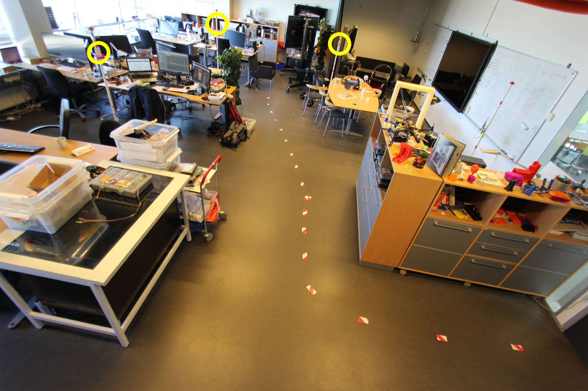Figure 4.1: Testbed at PitLAB, the yellow  circles indicate three trackable objects. In this picture we  want to  demonstrate how  things look  in  PitLAB and some of the trackable object’s true positions. In our  experiment we use  only  one  trackable object.

4.1    Experimental Setup

The  setup of the  system, means having 14 iBeacons mounted with fixed positions of X and Y  axis (all distances are demonstrated in figure  4.4) in relatively equal distance distribution of each axis.  The height of the iBeacons from  the floor is around

2100-2300mm this is hence to room structure and furniture 4.2.

The  idea  is that the  user has  a smartphone with our  Mobile Client application running on it. The user lets the smartphone collects data form the surrounding iBeacons like the  RSSI-values and UUID/MAC address.  The system then uses  RSSI data to predict the position of the smartphone in the room.

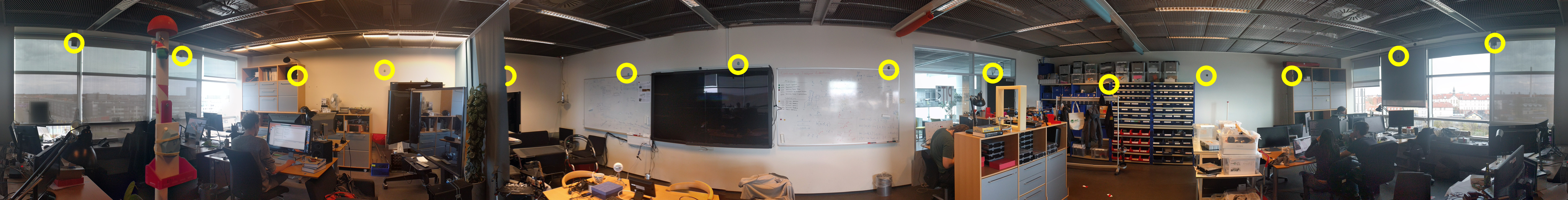Figure 4.2: PitLAB Panoramic view, a scale image version of this is in appendix chapter. If we zoom in the  image we can  see  the  nature of PitLAB. People, furniture in different heights, work-space and desks etc.

4.1.1    Trackable object

We use the same iBeacon type for our trackable object, the only different is our trackable  object does not  have  a fixed  position.  The  height of the  iBeacon is 1200mm mounted on an retried flag pole  4.3.

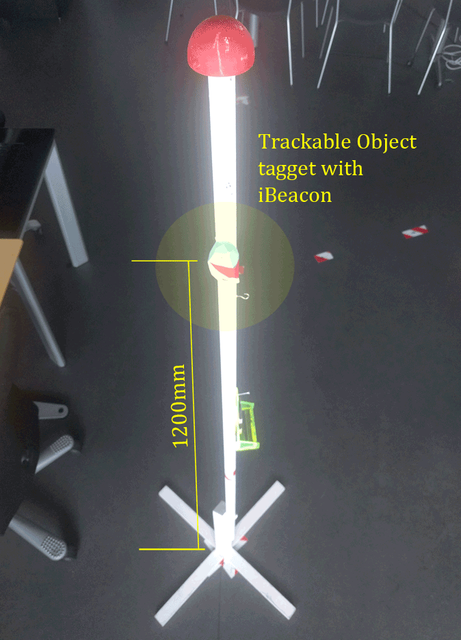Figure 4.3: Trackable object (Pole)  tag with  iBeacon. We asked the  Facility Management department of the IT-University if they could provide a pole  for testing, and luckily they had some old flag poles which have  been used throughout the study.

Figure 4.4: iBeacon fixed position in room. Here we show the  PitLAB room top  view and how 14 iBeacons with fixed positions are placed in the room

4.1.2    iBeacon specification

All our  iBeacons are  Estimote 4.5 brand. The two most important configuration of iBeacons is transmitting power (TxPower) and advertising period. TxPower is set to

-12dB and advertising is set to 967ms on all iBeacons.

Figure 4.5: Estimote iBeacons

4.1.3    Smartphone

The smartphone is from  Google, model LG Nexus 5x. Regarding to recent research made by Fürst [7], the  IT-University, this smartphone  should be the best phone to receive iBeacon signals. It makes it a suitable choice for our project.

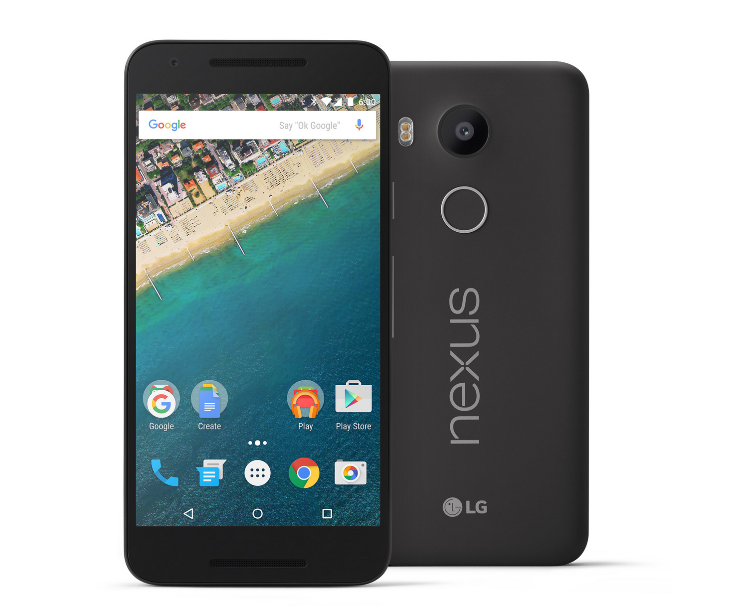Figure 4.6: Google Nexus 5X

4.2    Experiment

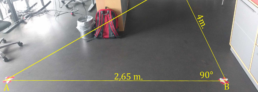
We mark the  floor  with four  positions, called true positions: A, B, C and D. At each true position we have four directions: 0, 90, 180 and 270 degrees, 0 is almost on Earth North direction, as demonstrated in picture 4.8.

We collect data from  all iBeacons (fixed  position iBeacons and trackable object iBeacon) from  each direction over  60 seconds of time. We hold the smartphone in our  hand, centered to the body front as demonstrated in the picture 4.8. We repeat this in four rounds.

For instance if the trackable object is placed on C, we collect data from  true position A Round 1 and true position B Round 2 from all directions. We continue to move the trackable object to D, and collect from true position B Round 1 and true position C Round 2 until trackable object has been through all true positions as shown in the experiment table 4.7.

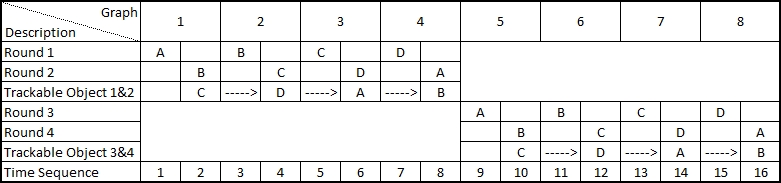Figure 4.7: This table presents rounds and the time sequence. Round 1 and Round 2 are parallel rounds, but  if we predict smartphone at A and predict smartphone at B, we predict trackable object at C. Later in this section eight different graphs will be presented (Graph1 to Graph8). These represent the results of the experiments.

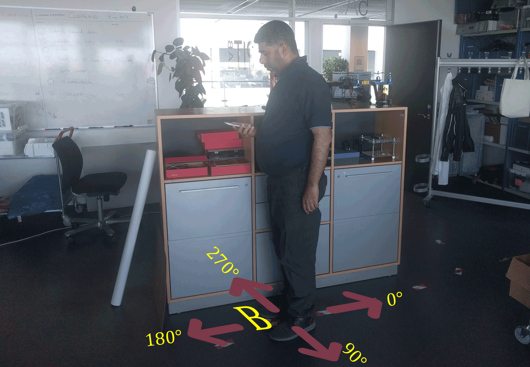Figure 4.8: A person holding smartphone testing RSSI receiving signals at Round 3 in true position B on angle 180° direction.

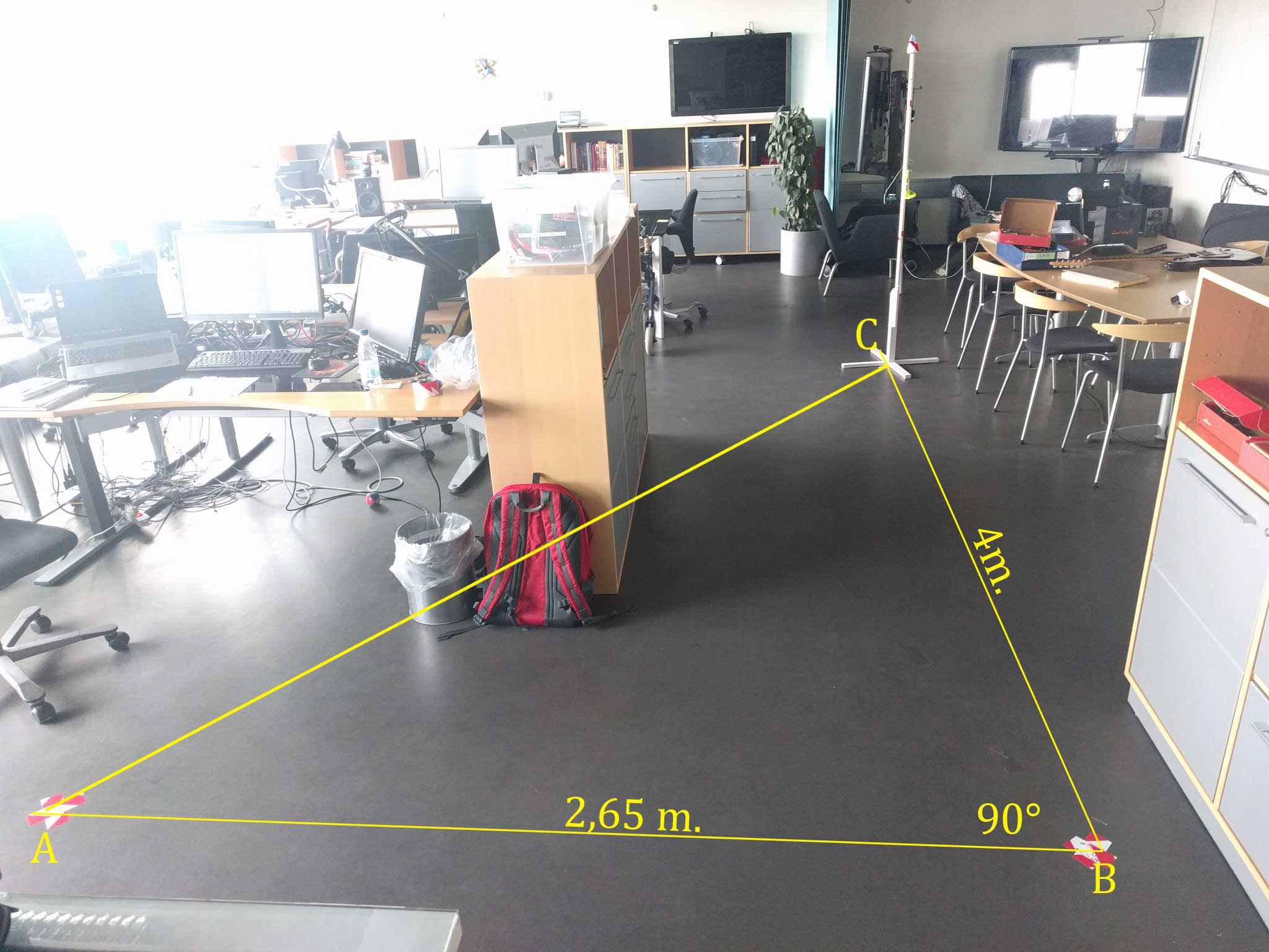Figure 4.9:  Testbed at PitLAB. We show here for instance Round 3, where the  user test smartphone at true position A and move to true position B to predict trackable object at true position C

4.3    Results and analysis

In experiments from  Round 1 and Round 2, we have totally 19 trackable objects estimation results and Round 3 and Round 4 from 23 trackable object estimation results. The  Red  mark belongs to true position C, Green belongs to true position D, Blue belongs to true position A and Orange belongs to true position B. For each colour cluster, we calculate a centroid of the collect data and represent this in bigger circle. We have  added a horizontal and vertical line in centre of our  graph in which each true position gets its own region respectively region AR, BR, CR and DR. The cross (+ sign)  in graph represent the true position of the trackable object as demonstrate in graph 4.10 and graph 4.11.

As it appears for Round 1 and 2, the position of Red centroid belongs to CR region, Green belong to DR, Blue belongs to AR, expect the last one  Orange which belongs to AR. However, Round 3 and 4, all colour belong to  their respective regions (we calculate our centroid by taking the average of x and y for each cluster).

Graph 1 4.10 shows the  result from  Round 1 and 2 and Graph 2 4.11 show the result of round 3 and 4.

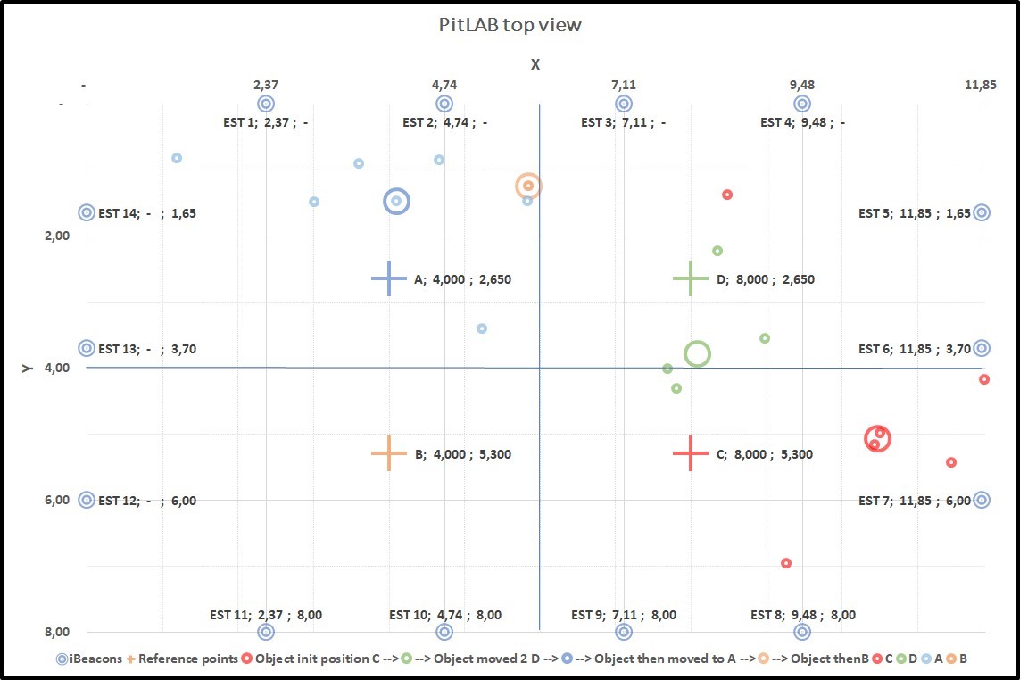Figure 4.10:  Round 1 and 2, (+) sign  represent true positions of trackable object, small dot  in graph represent trackable object estimation results over  time and the bigger circle  is a centroid product of the small dot cluster

Figure 4.11:  Round 3 and 4, (+) sign  represent true positions of trackable object, small dot  in graph represent trackable object estimation results over time and the bigger circle  is a centroid product of the small dot cluster

As explained in the beginning of this section, we predict a smartphone position at different angles in different true positions. For instance, we predict a smartphone at true position A and the same in true position B, then we use the results to calculate and predict the position of trackable object in C etc.

The  results from  the experiments are  presented in the  following eight different graphs. Each graph has two centroids of two predicted smartphone positions of four different directions with  cross (X) sign,  smartphones have  true positions with plus (+) sign,  small dots are generated by our  trilateration method from  combination of two predicted smartphone on different direction and a big circle  that represent the centroid of all small dots for trackable object.

Before  we start with  looking into the  eight graphs, we present a graph as an  example 4.12 and explain the signs:

+ sign: True  position
X sign:  Centroid of Smartphone predicted position
O sign:  Centroid of trackable object predicted position o sign:  Predicted positions of trackable object
A position top left
B position bottom left
C position bottom right
D position top right

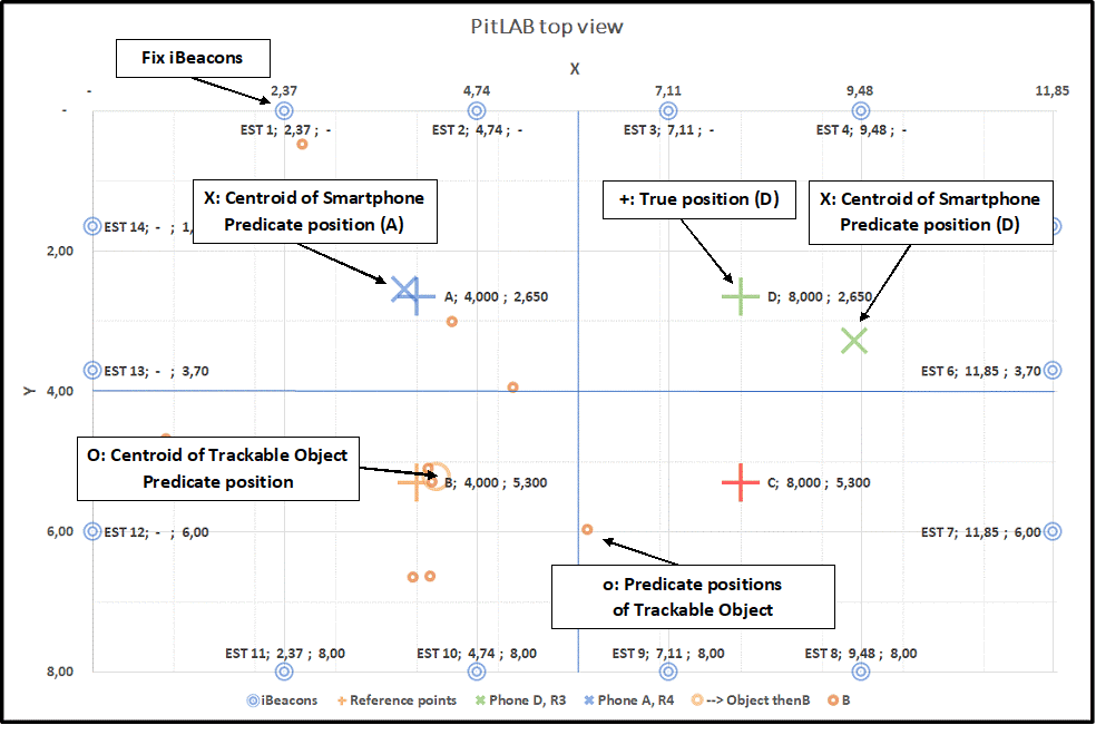Figure 4.12: Graph: This is a sample graph with explanation of different signs we use in the upcoming graphs.

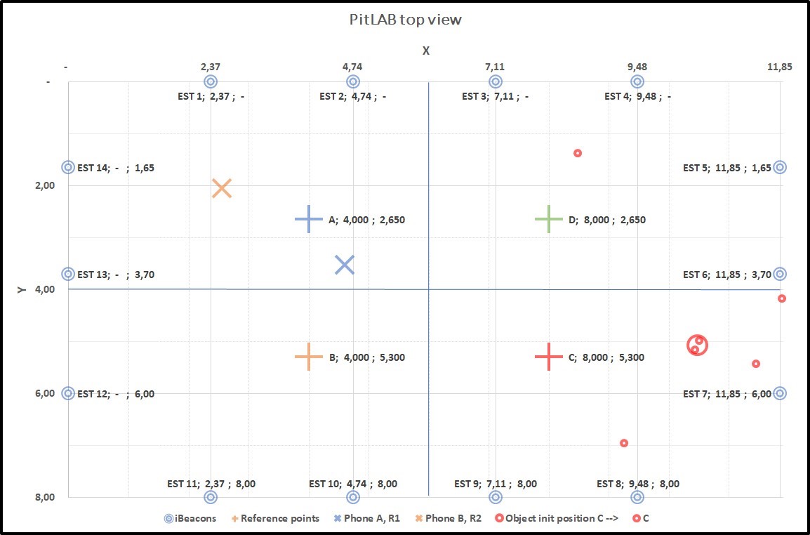Figure 4.13: Graph1: Collecting data from two true positions A(+) and B(+). A(X) and B(X) smartphone predicted position, B(X) is far away from  B(+), result of this predict position of trackable object centroid C(O) with true position of C(+)

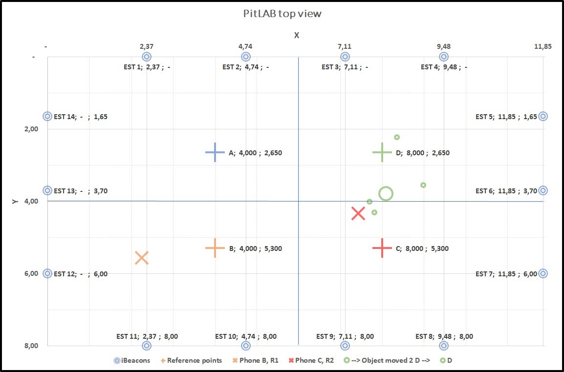Figure 4.14: Graph2: Collecting data from two true positions B(+) and C(+). B(X) and C(X) smartphone predicted position, result of this predicted position of trackable object centroid D(O) with true position of D(+)

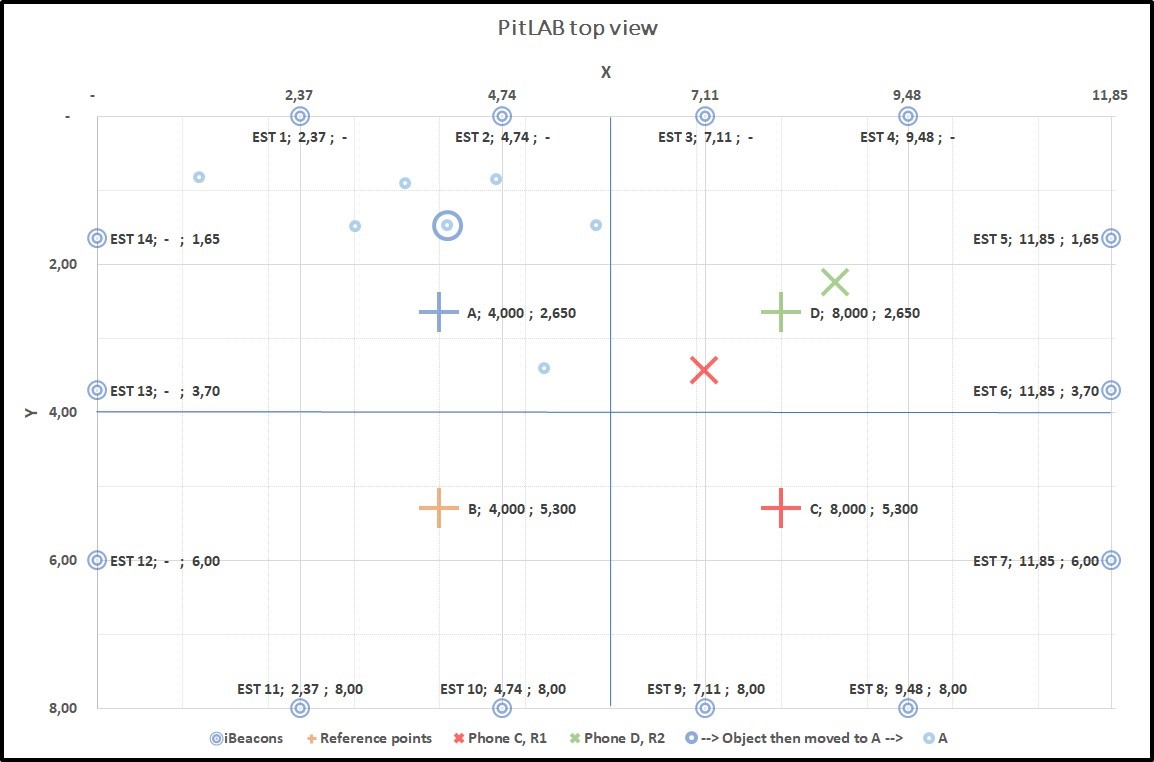Figure 4.15:  Graph3: Collecting data from  two true position C(+) and D(+).   C(X) and D(X) smartphone predicted position, C(X) is far away  from  C(+), result of this predicted position of trackable object centroid A(O) with true position of A(+)

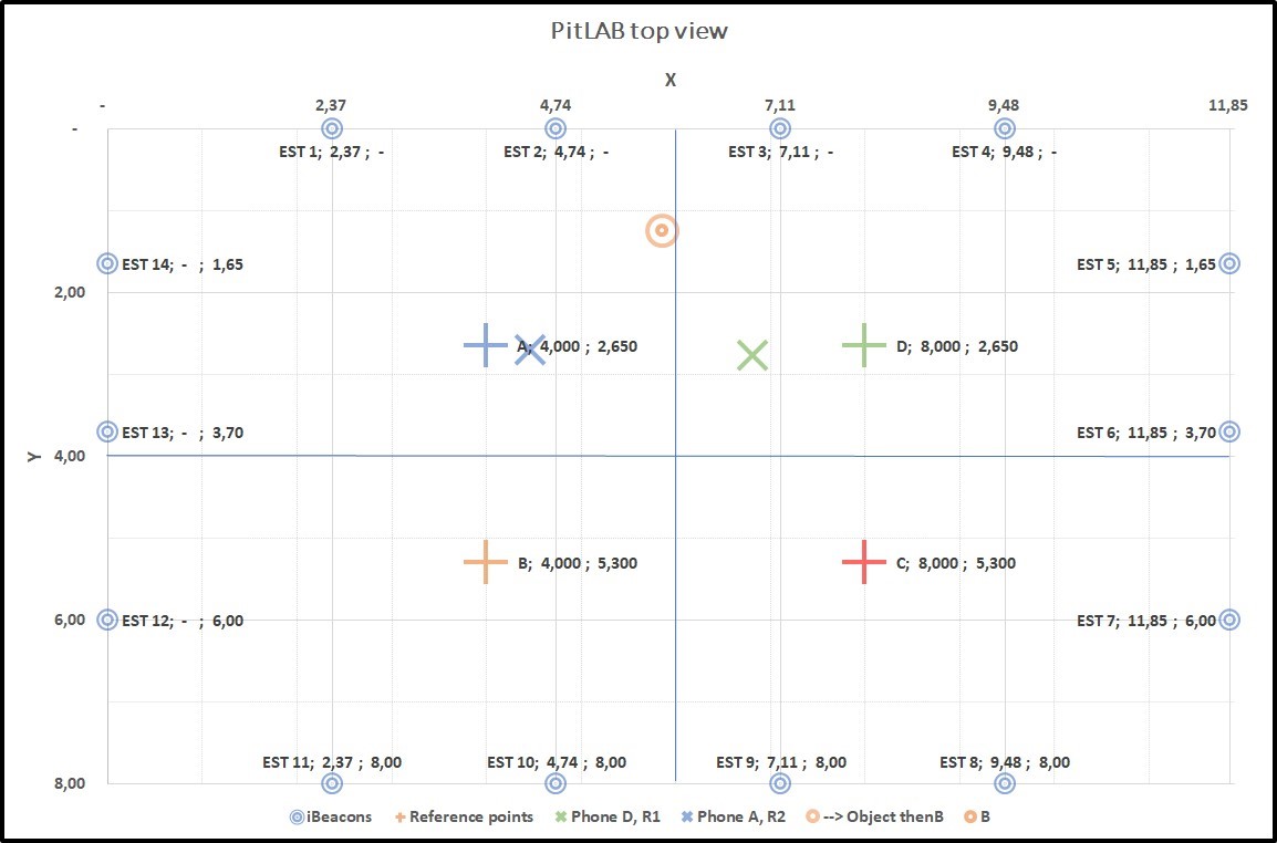Figure 4.16:  Graph4: Collecting data from  two true positions D(+) and A(+).  D(X) and A(X) smartphone predicted position, result of this  predicted position of trackable  object centroid A(O) with true position of B(+), Our algorithm was only able  to predict one  position

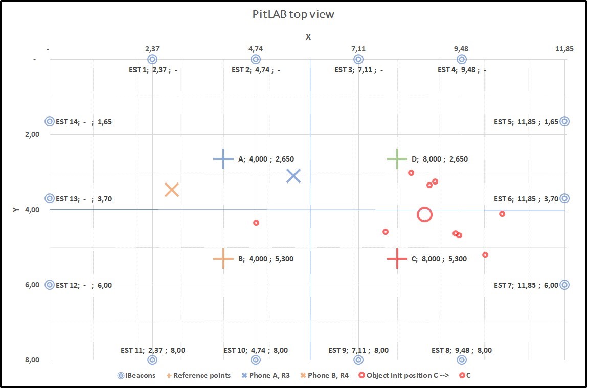Figure 4.17:  Graph5: Collecting data from  two true positions A(+) and B(+).  A(X) and B(X) smartphone predicted position, B(X) is far a way from  B(+), result of this predicted position of trackable object centroid C(O) with true position of C(+)

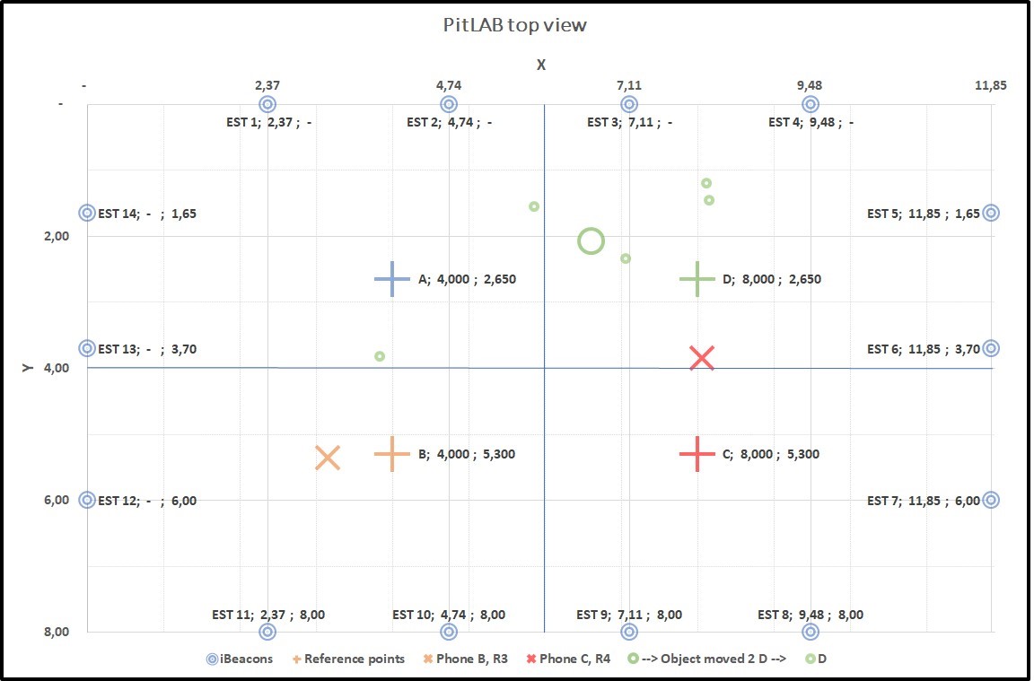Figure 4.18:  Graph6: Collecting data from  two true positions B(+) and C(+).  B(X) and C(X) smartphone predicted position, C(X) is far away  from  C(+), result of this predicted position of trackable object centroid D(O) with true position of D(+)

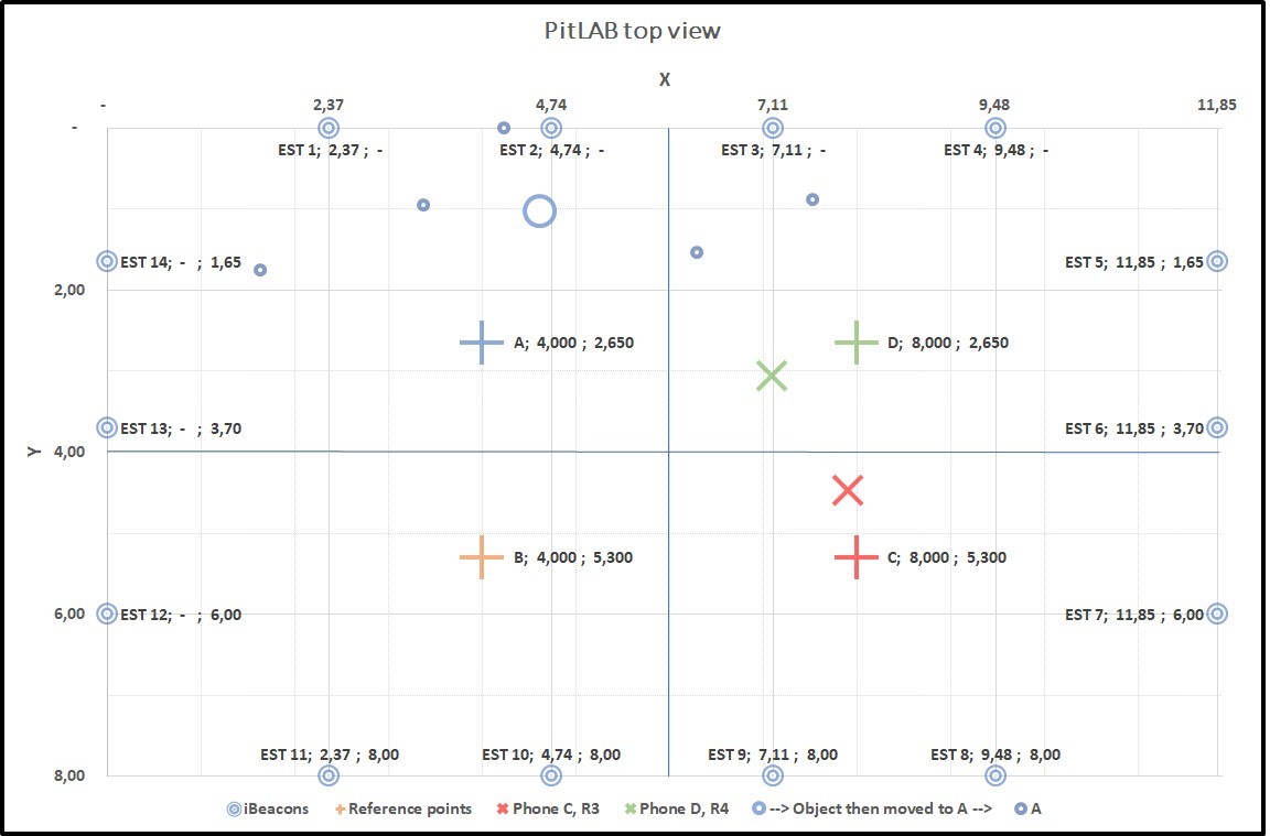Figure 4.19: Graph7: Collecting data from two true positions C(+) and D(+). C(X) and D(X) smartphone predicted position, result of this  predicted position of trackable object centroid A(O) with true position of A(+)

Figure 4.20: Graph8: Collecting data from two true positions D(+) and A(+). D(X) and A(X) smartphone predicted position, result of this predicted position of trackable object centroid B(O) with true position of B(+)

Since  we have  an average error level of 2.04 meter 4.4 with standard deviation of 0.28 meter 4.4, so if we want to visualize trackable object position on a map it would be much better to present it in a more human friendly and readable way.

In our  map, we have  four  true positions. If we split  the room horizontally and vertically in half, this would give use four regions, where each true position belongs to its respective region as described earlier.

The  same convention is used as before AR, BR, CR and DR. AR stays  for A Region,  B Region, etc.  If we take the trackable object position result from  the  previous graphs, then we can present the trackable object position in its region and its movement over time. As we can see in the first graph the trackable object has moved over time from  C to D, D to A and A to B is its final move.

In the  first graph, we see trackable object move over time on the respective path, expect A to B. If we look back in Graph4 4.16, we can see we have only one dot, where we normally should have  at least more than one  dot  as shown in graph 4.21.  Our system has  failed  to calculate the  results of the  particular place. The reason for this can vary, but  one  reason might be that the  particular time there could be affecting heavily with noise.

If we take  the  next  graph, the  trackable object follows  the path as expected as shown in graph 4.22.

Depending on the room size and the  error level, we assume it is possible to split the room in more regions to get smoother results. That  said,  we conclude that continues data collecting from  more phones over time will improve accuracy of the prediction of position results.

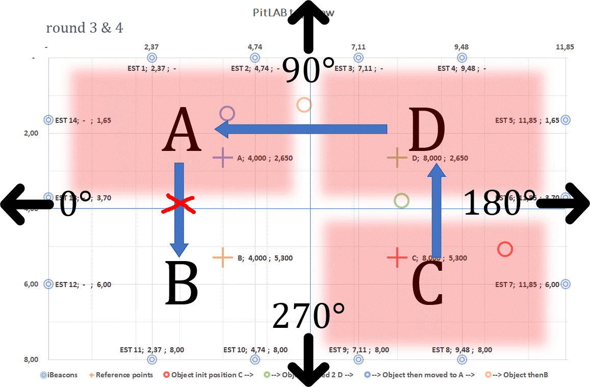Figure 4.21:  In this  graph we illustrate trackable object location in regions and its movement from  place to place over  time. This is a result of combination of Round 1 and 2. As we can  see the trackable object suppose to move to B region, since our system fails to calculate the results. This means trackable objects stop at A region

Figure 4.22:  In this  graph we illustrate trackable object location in regions and its movement from  place to place over time. This is a result of combination of Round 3 and 4.

4.4    Error level

We have  in chapter 2 under section RSSI measurement 2.2.2 talked about iBeacon and smartphone challenges and in same chapter talked about RSSI distance calculation 2.8 which shows the measuring errors over distance of our iBeacon. If we take all that into consideration and look at our results we discover an error margin in our results as well.

We have  made two  graphs to  illustrate the  error level  of our  system.  The  first graph demonstrates error level  of a smartphone.  We present the results of each Round and for each true position point in table. Then we calculate the hypotenuse of X and Y  to get the distance of the  error and present that in Cumulative distribution function (CDF) graph 4.24. We can  see that our overall results have  distribution of error at different levels but interesting enough that almost 75% of the results have error level below 1.5 meter with  average of 1.33 meter error and standard deviation of 0.13 meter.

However, in the Cumulative distribution function (CDF) graph 4.26, for trackable object, we can see the error average has raised to 2.04 meter with standard deviation of 0.28 meter. The interesting aspect of this graph is that 75% of the results are below 2 meter.

If we compare the error of trackable object to our  smartphone, we see the  trackable  object error level is higher than the one  from  smartphones. This is due t nature results, hence the trackable object get its position result from  smartphone positions which already have  error margin.

We calculate the hypotenuse with the following formula: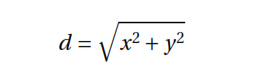d = error distance from  true position.

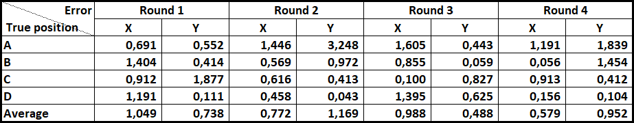Figure 4.23:  Smartphone distance error of each axis x and y for each true position and for each round, with average value  of each round.

Figure 4.24: CDF graph for smartphone distance error of hypotenuse results from  x and y from  previous table for each round

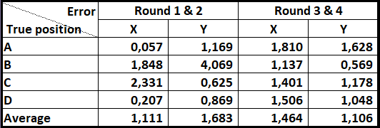Figure 4.25: Trackable object distance error of each axis x and y for each true position and for each combined rounds, with average value  of each round.

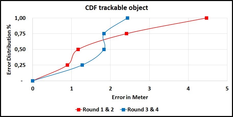Figure 4.26: CDF graph for trackable object error of hypotenuse results from  x and y from  previous table for each combined rounds.

4.5    Conclusion of this chapter

We conclude that BLE signals in iBeacon is hard to control. Even Estimote (the company that produces iBeacon, which we use in our  experiment) mention the issue of precision on their website 1. It is around 20-30%.  This said,  we cannot control the behaviour of BLE nature. In addition, we have learned that we need to predict a high number of smartphone position before we can  predict our  trackable object. However,  by developing and improving algorithms, we will be  able  to get some useful results.