
System Design
In this chapter, we will explain the system design behind Indoor Equipment Localization System (IELS).
Before we go into the details of the system, the main goals of this project will be elaborated. The following questions are chosen in order to create a direction for the project:
- Q: What is our goal?
A: To localize object in room. - Q: What do we need in order to localize object?
A: Some reference positions. - Q: How to get reference positions?
A: Some localization techniques like Trilateration. - Q: What does Trilateration need?
A: At least 2-3 Distances. - Q: How do we achieve distance?
A: One way is to convert RSSI values to distance. - Q: How do we get the best values?
A: by sorting strongest RSSI values.
These questions guided us to solve small problems that might be in a chain of a bigger problem. It helped as well to make some useful choices in our algorithm development.
In next section it is explained how our algorithm works and then take the elements that is involved in its development.
2.1. The Logic of the chosen Algorithm
The algorithm pseudo 1 is used for calculating the location of a smartphone that we use to calculate our trackable object location. Each step that has correlated processes and dependable methods will be explained later in this chapter.
In the infrastructure of the system, we use 14 iBeacons with fixed position and one iBeacon as trackable object as described in our evaluation experimental setup section. We use one mobile smartphone to collect our iBeacon data.
While we implemented our algorithm, we made regularly small tests, experiments and trail and fail, until we reached our solution. Conceptually one of the research papers gave us interesting knowledge about our Algorithm by Jea-Gu Lee who is mentioned in our Related Work-section. The main difference is that they use Double Gaussian Filter in their approach. In addition, some inspiration came from a previous work of Wouter Bulten.
In our approach, we collected all reachable iBeacons RSSI values over time and sort RSSI values in a descending order for each second. Then we take the three strongest RSSI values and convert those to the distance. Finally, by using trilateration mathematical equation we predict the estimate position of x- and y-coordinate of the mobile smartphone.
When we predict positions, we use the positions to calculate the position of our trackable object. A simplify example illustrate how our algorithm works to predict the estimated position of a trackable object in a room(see figure 2.1). When we collect more than one reference point like ’User A’ with a smartphone, we get estimate position A and estimate distance to trackable object (X1, Y1, d1). At some point, another user, ’User B’, with another smartphone get estimate position B and estimate distance to trackable object (X2, Y2, d2). This is the minimum information we need in order to calculate and predict the estimated position of a trackable object (X object, Y object). Our algorithm is used to predict an estimated position of a smartphone location over time and we use that information to calculate the estimate position of a trackable object.
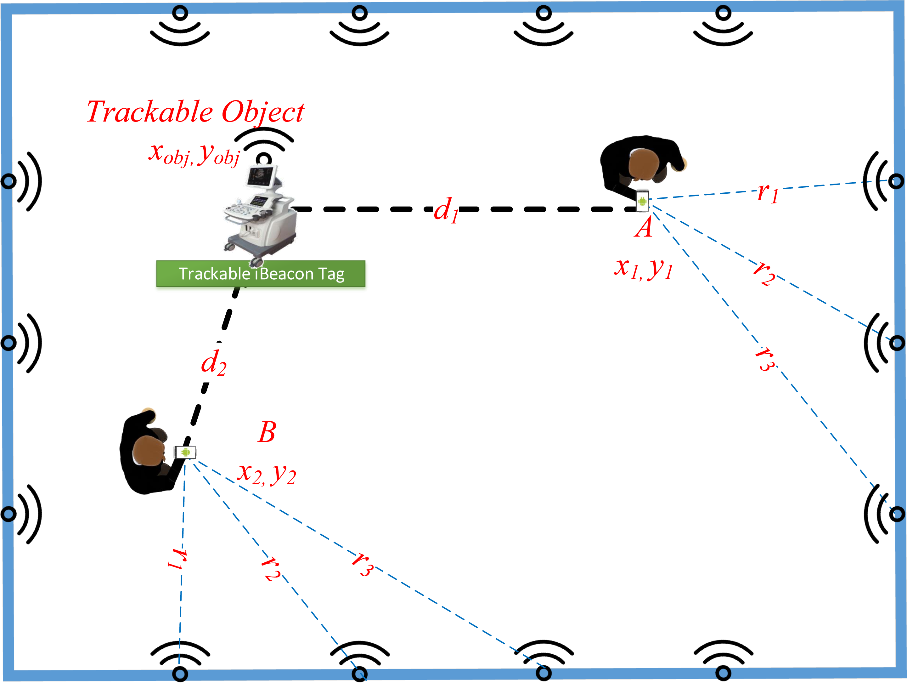 Figure 2.1: How to estimate a position of a trackable object from User A and User B.
In the previous section we explained the concept of our algorithm. In the following description we present the pseudo 1 code of the used algorithm.
Init Map Device Data Structure
Collect iBeacon RSSI
initTimeSeries {keep RSSI last value until updated}
kalman {Kalman filter RSSI for each iBeacon}
results {Moving Average of each kalman results}
bestRSSI {Sort results select best 3 RSSI each second}
(Note: Sort RSSI value descending order)

For each rssi set of $bestRSSI$ compute $DISTANCE(RSSI)$

If {at least 3 distance available}
    Return {$positionXY$($x_1$, $y_1$, $d_1$...$x_n$, $y_n$, $d_n$)} Else
    Return {no results}
EndIf

Procedure{distance}{$RSSI$}
    Compute RSSI to Distance
    Return $distance$
EndProcedure

Procedure{positionXY}{$x_1$, $y_1$, $d_1$...$x_n$, $y_n$, $d_n$}
    Compute using Trilateration
    Return $x_{new}$, $y_{new}$
EndProcedure
Initially, we initialize the data structure that contains all initial information aboutour fix iBeacon position, trackable object and mobile smartphone. The system then collects RSSI-values from all iBeacons (fix iBeacons and track-able object iBeacons). Our initTimeSeries will keep last RSSI-value until a new value is received. This isto guaranty that all iBeacons have values we can use for calculation.Afterwards, RSSI-values unfortunately includes noise (we will explain noise prob-lem later in this chapter), but with the use of a Kalman filter, it is possible to take theraw values and try to decrease the noise from the values and thereby predict newvalues. We take values from the Kalman filter and run it through moving averagefilter to smooth the RSSI-values.Finally, we sort RSSI-values and take the three strongest values for each second.
Now for each of these strong RSSI-values we use distance method to convert RSSI to distance. If there is at least three distances then we calculate location x and y.
2.2. Proximity distance estimation
As we mention in chapter 1, localization proximity is about having distance estimation between two objects, for instance smartphone receive iBeacon (RSSI-values)signal in dB (Decibel). This said, higher dB-values means stronger signal, which means shorter distanceto the sender-device. We allow us to transform this relation of dB-value to estimatedistance between sender- and receiver-device. There are a variety of methods forthis. In this thesis we mention three methods in section. There are various reason why distance estimation cannot be 100% accurate, suchas different types of obstacles as explained in paek paper page 7, section 4.7. The following section will introduce some distance estimation in more details.
2.2.1. Indoor Distance Estimation using RSSI signals
The nature of iBeacon RSSI-signals are unfortunately rather inaccurate, unstableand contains noise. Many factors play a role in fluctuation of RSSI-values; for in-stance, obstacles like: human movement, human body, type of wall, type of materi-als and other external noise factors etc.
In addition, each smartphone model and type has different BLE receiver, thatbehave differently from phone to phone.
Therefore, it is important to have a revision of measured RSSI-values for each en-vironment and each smartphone before using them as mentioned by Lee. Fromthis we can build a data model for each environment and smartphone type whichwe will describe in this section 2.2.2.1.
Regarding materials type that influence RSSI-signal, a paper by paek mentionthis problem in page 7, section 4.7. They solve this by building a data model for it.
2.2.2. RSSI measurement
As describe earlier in our algorithm logic, we need to estimate distance to calculatethe estimated position. In our case distance comes from RSSI-signal strength. Wewant to measure and understand the relation between RSSI and distance. This said,it is important to validate this and put that in a model so we can use it in our algo-rithm.
For this experiment, we use Estimote iBeacon (in the yellow circle) as a sendersource and LG Nexus 5X smartphone (below the half yellow circle) as a receiver.
We mark the floor with read/white lines indicating real distances from 0 to 30 meteras shown in figure 2.2. This measurement take place in front of PitLAB, 5th floor atIT-University of Copenhagen.
We collect RSSI-values over 60 seconds as shown 2.3 and calculate the averagevalue of morning, noon and night. The reason we choose morning, noon and nightis because in previous tests we made, we can see different behaviour and results forRSSI-values in those parts of the day.
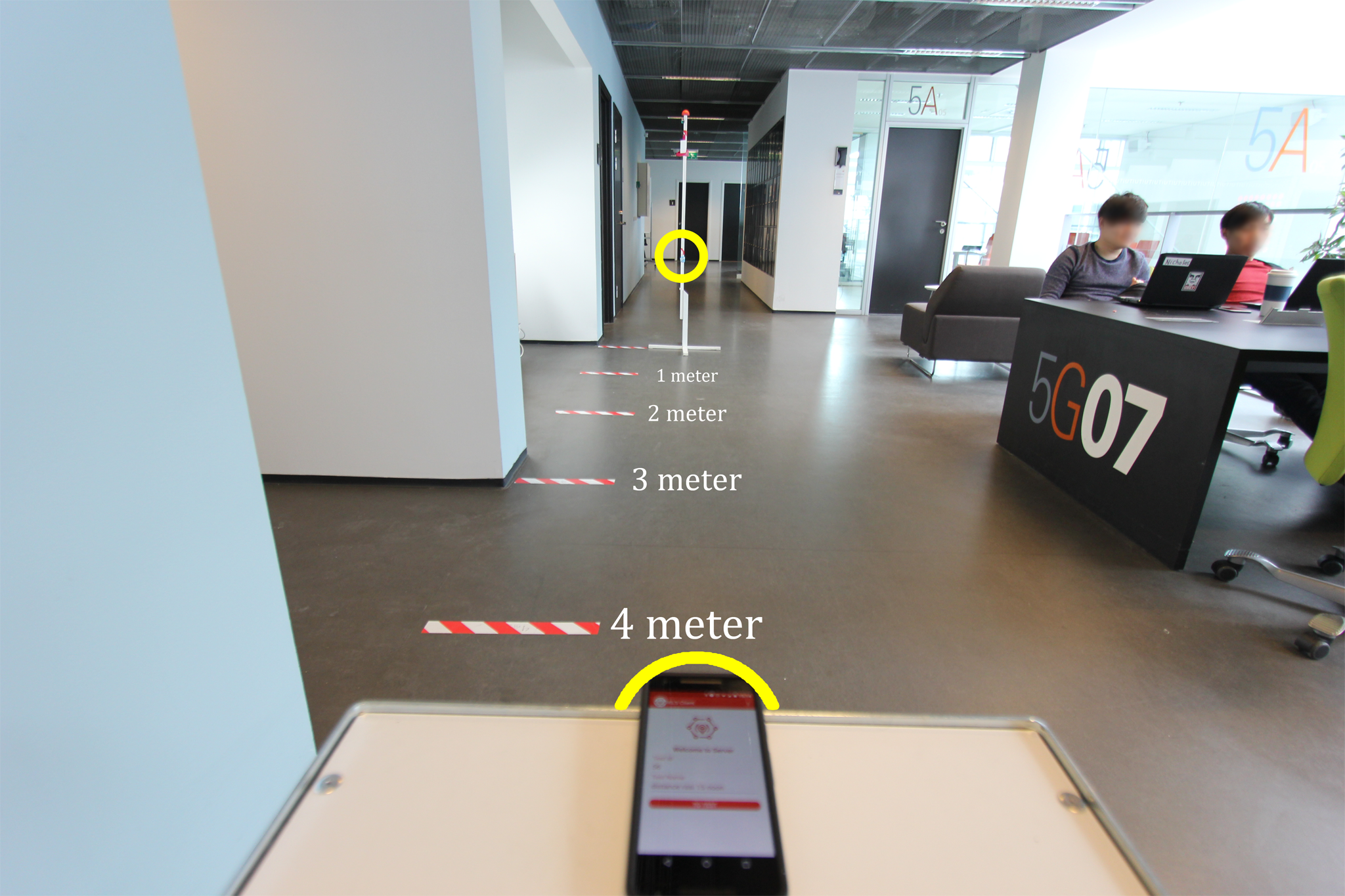 Figure 2.2: RSSI-value over distance measurement, in front of PitLAB
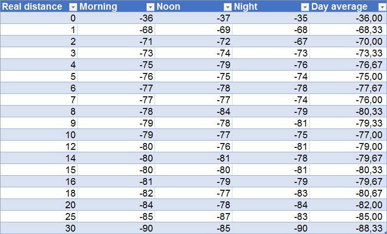 Figure 2.3: RSSI-values of morning, noon and night. All real distances are in metersand all RSSI-values in dB
Finally, the data is plotted in a graph 2.3, and the relation between distance andRSSI-values becomes clear. The results of the graph clearly shows a logarithmic cor-relation between signal-value over different distances in meter.
It is important to mention that RSSI-values can easily be affected by environment,signal-sources from other devices like Wi-Fi page 7 and obstacles page 8, hu-man body, walls etc. Even thus we have the smartphone and the iBeacon place ina fixed position. The importance of measurement gives us an approximate estima-tion of that particular environment and smartphone we use. Furthermore, the erroraverage increases as the distance increases as demonstrated in graph.
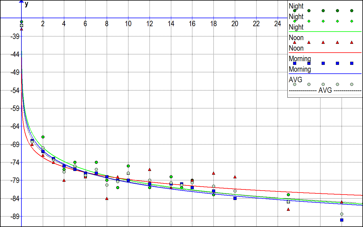 Figure 2.4: RSSI-value logarithmic correlation to distance. X: real distance in meter,Y: measured RSSI-value
2.2.2.1 Different smartphones challenge
From our tests and observation, we found that different smartphones have differentreading of RSSI-signal strength value and are not equal with latency. Latency in thiscontext is how many RSSI samples are received per second.
In addition, we observed also that smartphones behave differently in morningand evening time. For instance, the same smartphone with the same software cancollect up 3-4 samples per second in the evening hours and only one in the morn-ing or noon. The reason for this can be many, but one might be noise generatedfrom other sources such as Wi-Fi-usage in open hours. This said, it is unclear whatcaused this behaviour. Interesting enough while we worked with these challenges,a recently published paper from Fürst mentioned some of these challenges. Wehave added a minor supportive arm to some of the experiments in this paper asshown in figure 2.5. The measurement shows different results from different smart-phones as shown in the chart.
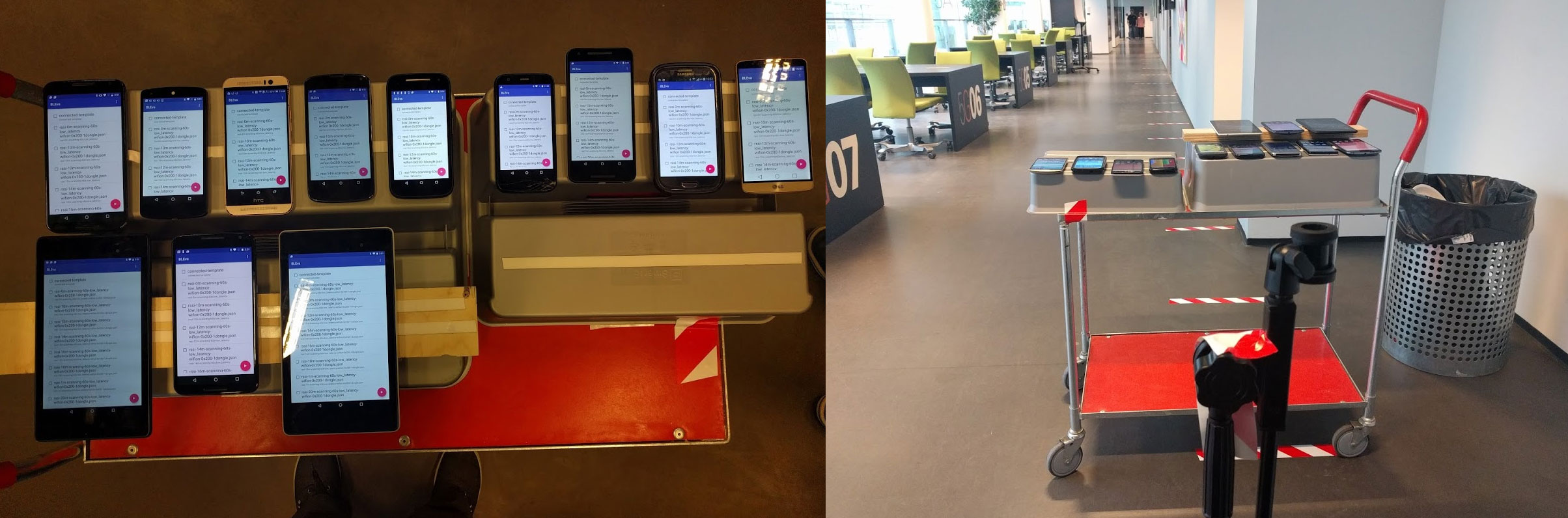 Figure 2.5: Smartphones comparison, collecting RSSI-values from same source. Ex-periments from the following paper
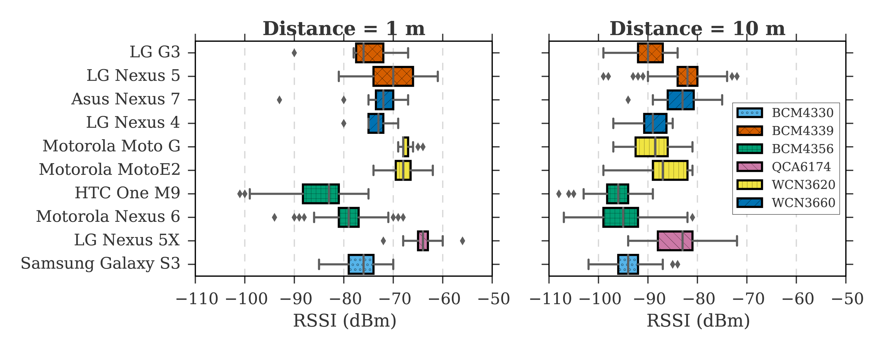 Figure 2.6: RSSI variation between different smartphone models from paper
2.2.3. RSSI distance calculation
We built a data model for our RSSI-value over distance in meter, but have can wecalculate RSSI-values to distance? There are many ways to calculate the estimateddistance between iBeacon sender- and phone-receiver using the RSSI-values.
In our design we experiment with three different methods, and make a compari-son chart 2.7 between the results.
For the following methods the iBeacon txPower (txPower stays for BroadcastingPower or Transmission Power of iBeacon) was set to -12dB and advertising rate is setto 967ms:
1- Generic log distance. . . is a generic method that is known to be used inmeasuring distance based on RSSI-values. The method results depending oniBeacon transmission power and a free space factor value which is normally between 2 and 4, in this experiment we used -12dB txPower which is the de-fault value by Estimote and the free space factor was set lower than 2 hence toreduce error scale: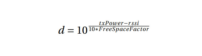
txPower = transmiton power of iBeacon
RSSI = value of signal strength
Free Space Factor = a value between 2 and 4
2- Estimote. . . is mentioned in two research papers”An Analysis of the Accuracyof Bluetooth Low Energy for Indoor Positioning Application”and”A Mea-surement Study of BLE iBeacon and Geometric Adjustment Scheme for IndoorLocation-Based Mobile Applications”.The same method is used and supported by Estimote beacons. It issimilar to previous method but the factor is set to a fixed value two. The mathformula for this method is: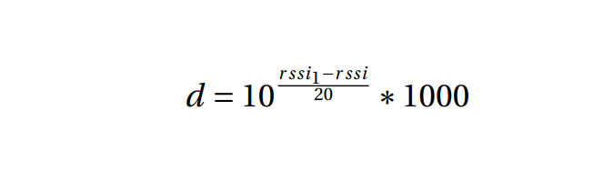
rssi1= RSSI is measured in 1 meter, in our case it was -68dB
The final result is multiplied by 1000 to get results in Millimeter.
3- AltBeacon. . . is based on AltBeacon library and is used in a paper”An IndoorPositioning Algorithm Using Bluetooth Low Energy RSSI” with followingmath formula:
![]()
The numbers 0.89976, 7.7095 and 0.111 are constant values set by the devel-oper of this method with out further explanation.The final result is divided by 1000 to get results in millimeter.
NOTE: All mentioned methods in our RSSI distance calculation section returnresults in millimeter unit.
We test all above mentioned methods in Excel and Java, the result of all methodsare presented in graph 2.7 shows conversion of RSSI to meter for each distance.
The results clearly shows from figure 2.7 and error figure 2.8 that Method 1 has least errors, and Method 3 has most errors in our LG Nexus 5x smartphone.
It is clear that RSSI do not increase linearly with distance, the error margin in-creases as the distance increases. That said, all this can change from place to place,depending on the noise and distortion on that particular environment, but the log-arithmic correlation would still hold on all environment.
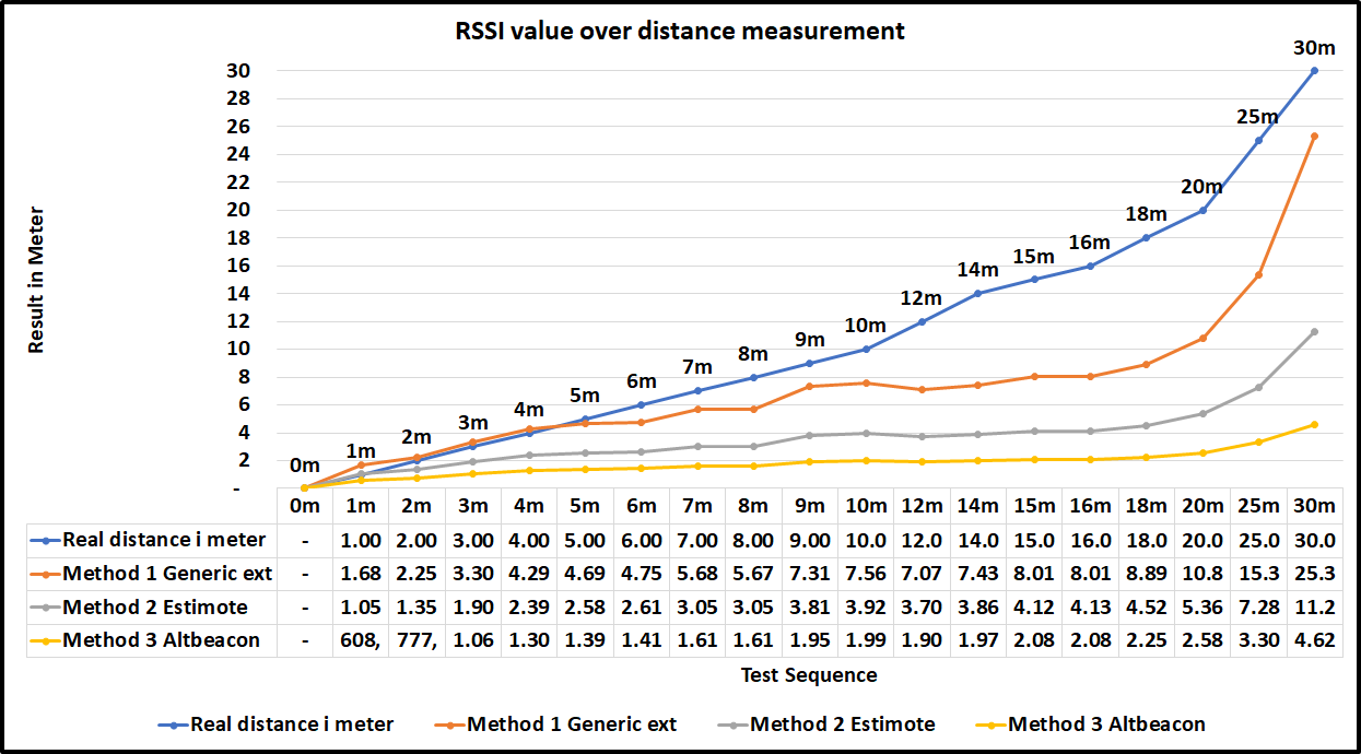 Figure 2.7: RSSI over distance in meter comparison graph for different conversionmethods, X: Real distance in meter, Y: Measure distance in meter. The iBeacon tx-Power was set to -12dB with advertising rate is set to 967ms11
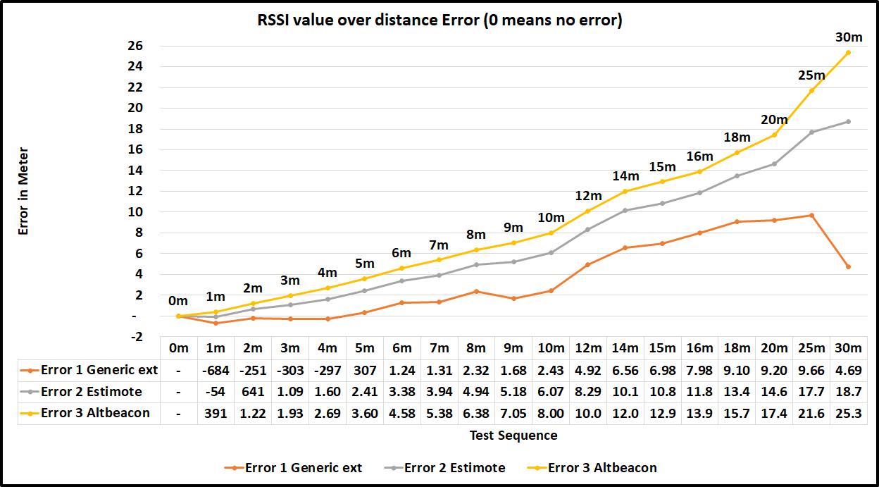 Figure 2.8: RSSI over distance in meter comparison graph for error level of differentconversion methods, X: Real distance in meter, Y: error level in meter. The iBeacontxPower was set to -12dB with advertising rate is set to 967ms
2.3. Time Series Processing
’Time series’ refers to a sequence of observations following each other in time, where adjacent observations are correlated. The main reason for using time series processing in our project is because we observed form early experiments that our raw RSSI-values contain noise over time. We have analyzed raw RSSI-values, as shown in oneexample in graph 2.9.
It is therefore obvious to work with time series processing methods. As men-tioned earlier, for various reasons, there will always be “noise” and “distortion” inwhen receiving a iBeacon RSSI-signal, even if the receiver is not moving. This wouldrequire a way of cleaning and processing strategies for time-series data.
The book Ubiquitous Computing Fundamentals shows various methods forhelping smoothing RSSI-values by filtering out the noise and distortion from differ-ent fluctuations. Time series models can be simulated, estimated from data, andused to produce forecasts of future behaviour.
In this project, we know that we have something to do with time series process-ing but was not sure which one and how to use. We gathered some basic knowledgefrom different resources (like previous works, Ubiquitous Computing and online re-search). Then we did a lot of trial and error, all ended up with using two popular filtering techniques: The Mean filter (Moving Average) and the Kalman filter.
2.3.1 Moving Average
Moving Average (MA) filter is a trend-following (trend in this context means a pat-tern of gradual change in a condition, output, or process, or an average or generaltendency of a series of data points to move in a certain direction over time2) be-cause it is based on past RSSI-values in this case. There are different types of movingaverage, the most common used Moving Average for this purpose is Simple Mov-ing Average (SMA), which is the simple average of a security spread across a definednumber of time periods. The most common applications of Moving Average are toidentify the trend direction and to determine signal level.
In our design, we implement a moving average and demonstrate the differencebetween our RSSI-input (black trend) and Average (green trend) output in figure 2.9.
The moving average takesnnumbers of RSSI-values, defined as window size. The method returns the average of RSSI-value of the given window size.
Our moving average implementation is based on following formula inspired fromJohn Krumm book Ubiquitous Computing Fundamentals  We have set our n value (window size) to be 10, we can see clearly this methodreduce some of the noise from the original input. We have tried different windowsizes, if window the size become five we get more noise in output and if we increaseit to 20-25, this will cost calculation delay of processing. It was decided to work withnumber ten to reach a balance value for this purpose.
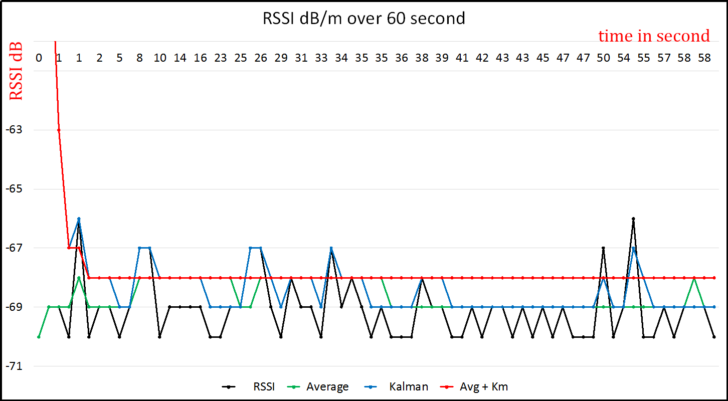 Figure 2.9: RSSI filter comparison, X: Time in Second, Y: RSSI value in dB
2.3.2 Kalman
Kalman filters will not be described in details, since there is a lot of papers and on-line resources describing Kalman filter. Roughly, we use Kalman filters to reduce thelarge spikes of RSSI-values as shown in graph 2.9, while trying to retain distance in-formation. A (regular) Kalman Filter is used to filter incoming signal strength mea-surement. The true RSSI-value (without noise) is defined as the state we want toestimate. Our Kalman filter implementation is based on existing pseudo-code of aprevious master thesis done by Mr. Wouter Bulten.
A Kalman filter returns RSSI-values as a Integers and we can see from the figure 2.9 that a Kalman filter reduces some of the noise from the original RSSI input.
2.3.3. Combining methods
From both observation we can see both methods reduce an amount of the noise.In this project we wanted to try to combine moving averages and Kalman filter toreduce the noise from RSSI-values as shown in figure 2.9. What we did is passing thelast measured result of the Kalman filter to the moving average of ten window size.This has reduced the noise drastically.
At an early stage we put the values into a spread sheet and made some primitivecalculation. Then we implemented a simple version of Moving Average that helped a bit to remove some of the noise, but not all of it. Later in the development processafter trying with different other methods, we tried to implement an already existingpseudo-code of a Kalman filter inspired from the master thesis by Mr. Wouter Bul-ten. The method did indeed remove some of the noise as well. We thought: ifboth filters remove some noise, it could perhaps be an option to combine the fil-ters – and the quality of the results increased significantly. One of the reasons our graph has a straight line is because we use Integer values which cleans up some ofthe noises as well.Nevertheless, this comes with a cost: Mostly, it takes up to 10 seconds before thesystem is able to calculate values.
2.4. Localization algorithms
There is different ways and methods to use for localizing – all depending on the out-come and the requirement of the project. As mention in chapter 1 there are sixmethods for localization and we have already defined the methods.
So far we have used proximity relation to RSSI over distance estimation. Now wewill use Trilateration in our algorithm hence we have a lot of distance andxandypositions. Hyperbolic lateration is more related to time of flight (TOF) techniquewhich is used in GPS-localization and Triangulation is typically used for high an-tenna tower. Fingerprinting and Dead reckoning might be relevant to our projectbut is left for the discussion-chapter.
Trilateration 2.10 is a mathematical equation that computesxandyposition ofa smartphone in our case, by calculating at least three distances to fixed positions ofxandy. Trilateration is able to calculate the position by using two distances insteadof three, but that will increase the error level which leads to reduction of accuracy.
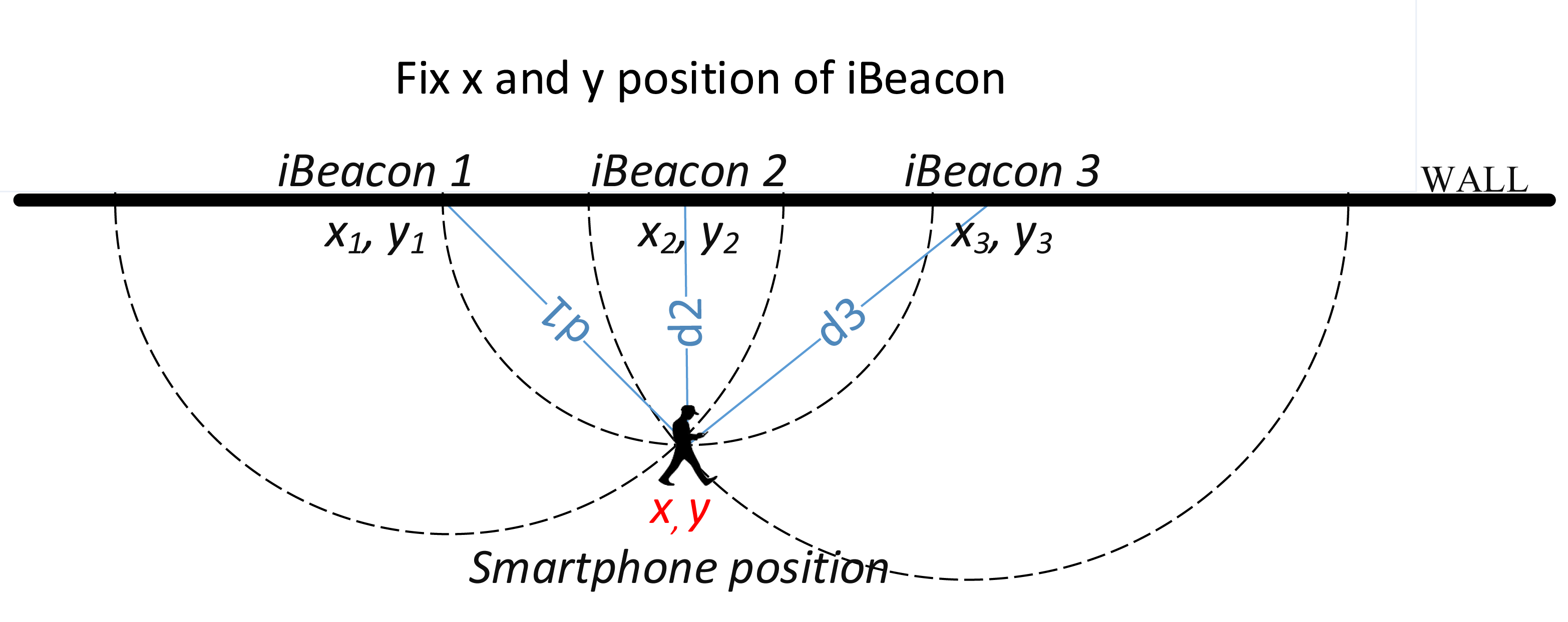 Figure 2.10: Illustrate how trilateration works
In our Algorithm, we use a Java-library called Lemmingapex trilateration. Wewanted to be sure that this library works correct. We injected different tests withthree positions and three distances and we got an expected results.
In addition, we have also chosen to implement a lightweight and static (static inthis context means sensitive for estimate distances) trilateration method for com-parison purpose, and we implemented a basic trilateration formula from The Uni-versity of Georgia3. The university provide a detailed explanation and sample excelfile with math formula. We have used the same test data from previous method andwe got close to identical results. Hence Lemmingapex has been used by some de-velopers and has better features then our basic implementation. It might take morethan three reference points and are more dynamic (dynamic in this context meansthe method is suited for handling estimated distances), we have therefore chosen tocontinue using the Lemmingapex-library in our implementation.
2.5. Conclusion of this chapter
In this chapter we presented different methods: distance estimation based on RSSI-values, moving average, Kalman filter and trilateration. All of them to calculate smartphone positions. The progress of this process relies heavily on previous work and achievements from other papers, inspiration from Ubiquitous Computing Fundamentals by Krumm, reverse engineering thinking and most importantly: trail and error. We conclude here that RSSI-values have logarithmic relation to distance as well as errors margin rise as the distance increases – and how RSSI is able to change values from surrounding environment and external factors. Finally, different smartphones type and models gives different results.